A comparative analysis is a significant process to compare two or more entities on the basis of specific parameters. We carry out comparative analysis by referring latest IEEE papers of that current year and also share the referred papers as per your needs. To carry out a WSN simulation comparative analysis, we provide a procedural flow by considering an instance as an assumption-based comparison among two routing protocols.
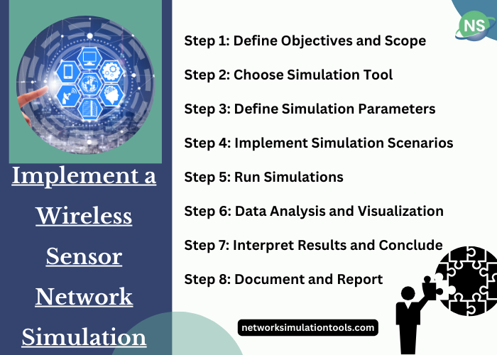
Step 1: Define Goals and Range
- Goal: First, consider Protocol A and Protocol B as an example of routing protocols. On the basis of latency, packet delivery ratio, and energy effectiveness, you need to decide which routing protocol offers efficient performance in WSN.
- Range: Based on a stable WSN with a determined number of sensor nodes and consistent distribution in a defined dimension of area, the comparison process will be constrained.
Step 2: Choose Simulation Tool
The simulation tool that you choose must aid the particular characteristics that are required for your analysis process and facilitate the WSN simulations. So, determine the tool accordingly. MATLAB as well as NS-2 could be appropriate for the process of comparative analysis that includes performance indicators and networking protocols, but it is based on the complex level of the routing protocols and your knowledge about these tools. Because of the NS-2’s wide range of assistance for networking protocols, consider you are choosing it for this instance.
Step 3: Define Simulation Parameters
- Network Topology: The number of nodes, node allocation, and dimension of area must be specified.
- Routing Protocols: Within the simulation platform, utilize or apply previous frameworks for Protocol A or Protocol B.
- Traffic Model: Describe the kind of traffic (for instance: constant bit rate) and the data generation rate at sensor nodes.
- Simulation Time: It is necessary to allot the time-limit of the simulation needed for gathering adequate data.
- Metrics for Comparison:
- Energy Effectiveness: It denotes the average energy that is utilized by each node.
- Latency: Latency indicates the average time that is required for the packet to travel from a node to the base station.
- Packet Delivery Ratio (PDR): PDR specifies the percentage of packets that are transmitted to the base station in an efficient manner.
Step 4: Implement Simulation Scenarios
- Scenario 1 (Protocol A): By assuring that all the parameters are stable, setup the simulation platform for Protocol A.
- Scenario 2 (Protocol B): In terms of the similar constraints, replicate the simulation setup with Protocol B.
Step 5: Run Simulations
By gathering all the data that are related to the specified indicators, run the simulations for Protocol A as well as Protocol B. To assure statistical relevance and to clarify differences, make sure whether each simulation has undergone several times of execution.
Step 6: Data Analysis and Visualization
To compare the efficiency of both Protocol A and Protocol B, examine the data that are gathered from the simulation processes. For identifying the importance of the outcomes, employ statistical analysis. To depict the comparative efficiency in an explicit manner, visualize the data through the utilization of charts and graphs. As an instance: use pie charts for packet delivery ratio, line graphs for latency over time, and bar charts for energy utilization.
Step 7: Interpret Results and Conclude
In terms of the specified range and goals, the outcomes have to be described. For each and every indicator, emphasize the protocol that achieves better results. It is also important to offer perceptions based on the reason behind the appropriateness of specific protocols for particular WSN-related constraints or applications. Any challenges or contradictions that are analyzed at the time of comparative process should be examined.
Step 8: Document and Report
By summarizing the major aspects of the comparative analysis such as methodology, simulation arrangements, outcomes, and conclusions, make an extensive depiction or documentation. Information relevant to the parameters, simulation platform and the considerations that are assumed has to be encompassed. For further exploration or the placements of WSN, describe the possible impacts of the discoveries.
How to simulate WSN in MATLAB?
Simulation of WSN in MATLAB is generally considered as an important as well as intriguing process and it is significant to follow major procedures and steps. Regarding this, we offer a simple instance below in a step-by-step manner that gives you a strong basis but does not include some latest characteristics such as complicated ecological communications or dynamic routing.
Step 1: Install MATLAB and Needed Toolboxes
It is crucial to make sure whether you have MATLAB that is installed in a proper manner, including all the required toolboxes. Specifically in WSN simulations, highly complicated simulations that encompass particular interaction protocols might be carried out with the help of Communications Toolbox.
Step 2: Define Network Parameters
Initially, your network parameters like the total count of nodes, size of the area, and the range of interaction for each and every node have to be specified explicitly.
% Network parameters
numNodes = 100; % Number of sensor nodes
areaSize = [200, 200]; % Area (m x m)
commRange = 30; % Communication range (m)
baseStation = [100, 100]; % Position of the base station
Step 3: Generate Node Positions
After that, allocate the sensor nodes across the defined area in a random way.
Randomly distribute the sensor nodes within the specified area.
% Generate random positions for nodes
nodePositions = areaSize .* rand(numNodes, 2);
Step 4: Plot the Network
To verify the location of the base station and the allocation of nodes, visualize the network.
figure;
plot(nodePositions(:,1), nodePositions(:,2), ‘b.’); hold on;
plot(baseStation(1), baseStation(2), ‘r^’, ‘MarkerSize’, 10, ‘LineWidth’, 2);
legend(‘Sensor Nodes’, ‘Base Station’);
title(‘Wireless Sensor Network Topology’);
xlabel(‘X position (m)’);
ylabel(‘Y position (m)’);
axis([0 areaSize(1) 0 areaSize(2)]);
grid on; box on;
Step 5: Simulate Simple Communication
If every node is within the range, infer that it transmits data to the base station. Note that intricate routing or real data packets are not encompassed by this instance.
% Calculate distance of each node from the base station
distances = sqrt(sum((nodePositions – baseStation).^2, 2));
% Determine if each node can communicate directly with the base station
canCommunicate = distances <= commRange;
% Count the number of nodes that can communicate
numCanCommunicate = sum(canCommunicate);
fprintf(‘%d out of %d nodes can communicate directly with the base station.\n’, numCanCommunicate, numNodes);
Step 6: Energy Consumption Model
On the basis of the node interaction with the base station, assess utilization of energy by using a basic model. For energy values, this instance employs a variable.
% Energy consumption parameters (placeholders)
energyPerCommunication = 1; % Energy used for communication
initialEnergy = 10; % Initial energy of each node
% Calculate energy consumption for each node
energyConsumed = initialEnergy – canCommunicate * energyPerCommunication;
% Display average remaining energy
avgRemainingEnergy = mean(energyConsumed);
fprintf(‘Average remaining energy: %.2f units\n’, avgRemainingEnergy);
Step 7: Analysis and Visualization
By concentrating on various indicators such as the average remaining energy and the percentage of nodes that are capable of interacting with the base station, the outcomes of your simulation have to be examined. If required, these outcomes can be visualized by means of histograms or plots.